데이터 전처리
- Null 처리
- 불필요한 속성 제거
- 레이블 인코딩 수행 = 간략하게 하기 위함
모델 학습 및 검증/예측/평가
- 모델 학습 : 결정트리, 랜덤포레스트, 로지스틱 회귀 학습 비교
- 검증 평가 : K-fold 교차 검증, cross_val_score(), GridSearchCV() 수행
1.1 데이터 확인
import numpy as np
import pandas as pd
import matplotlib.pyplot as plt
import seaborn as sns
%matplotlib inline
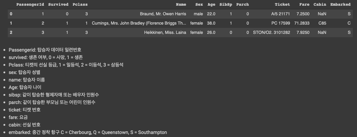
titanic_df = pd.read_csv('./titanic_train.csv')
titanic_df.head(3)
분석 시작 전 : 등급(높은 등급 먼저), 성별(여성), 나이(어린아이, 노약자) 가 중요할 것 같다고 판단된다.
1.2. Null값, 데이터타입 확인
print('\n ### train 데이터 정보 ###  \n')
print(titanic_df.info())
- null 칼럼은 대체를 할 것이고
- object 컬럼도 필요 없으면 drop 하고
- 카테고리성 컬럼은 레이블 인코딩을 진행한다.
1.3 NULL 처리
titanic_df['Age'].fillna(titanic_df['Age'].mean(),inplace=True)
# Age 컬럼에 해당되는 객체 자체를 평균값으로 업데이트 해준다. 그리고 대체한다.
titanic_df['Cabin'].fillna('N',inplace=True)
# 다른 카테고리성 컬럼인 N으로 대체한다.
titanic_df['Embarked'].fillna('N',inplace=True)

print('데이터 세트 Null 값 갯수 ',titanic_df.isnull().sum().sum())
# .isnull().sum() : 전체 칼럼별로 null 이 나옴
# .isnull().sum().sum() : 모든 컬럼의 null 개수가 나온다.


>> 데이터 세트 Null 값 갯수  0
Null 값 개수 확인하면 0이 나오는 거 확인할 수 있다.
print('데이터 세트 Null 값 갯수 ',titanic_df.isnull().sum())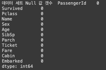
1.4. 데이터타입이 object 인 것들 : Sex, Cabin, Embarked 분포 확인 : value_counts()
print(' Sex 값 분포 :\n',titanic_df['Sex'].value_counts())
print('\n Cabin 값 분포 :\n',titanic_df['Cabin'].value_counts())
print('\n Embarked 값 분포 :\n',titanic_df['Embarked'].value_counts())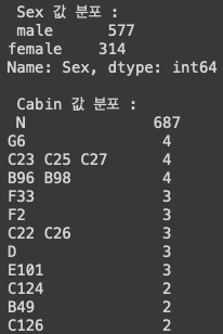

선실 등급만 가져가보자
titanic_df['Cabin'] = titanic_df['Cabin'].str[:1] # 등급별로 진행하기 위해 앞글자만 가지고 온다.
print(titanic_df['Cabin'].head(3)) # 3개만 가져와 보자
titanic_df['Cabin'].value_counts() # 분포도 확인
분포도를 확인하면 위와 같이 되어있는 것을 확인할 수 있다.
1.5. 성별별로 사망자와 생존자 분포 확인
titanic_df.groupby(['Sex','Survived'])['Survived'].count() # 성별별로 사망자, 생존자 확인
# Sex, Survived로 묶어준 후 Survived에 대해 카운트
1 : 생존, 0 : 사망
여성분들이 생존을 더 많이 한 것을 확인할 수 있다.
Seaborn 으로 시각화해보기
# seaborn 으로 시각화 해보기
sns.barplot(x='Sex', y = 'Survived', data=titanic_df)
# seaborn 에는 데이터 프레임이 들어오고 자기가 알아서 컬럼을 찾아서 x축 y축에 그려준다.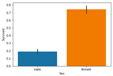
1.6. 선실 등급에 따른 생존자 분류
hue : 같이 비교해준다.
# 선실 등급에 따른 생존자 분류
sns.barplot(x='Pclass', y='Survived', hue='Sex', data=titanic_df) # hue에 해당되는 컬럼을 같이 비교해준다.
남성분들은 선실등급이 높을수록 생존 확률이 높았고
여성분들도 비슷하다.
1.7. 나이에 따른 생존자 분류
카테고리를 나눈 후에 진행
# 입력 age에 따라 구분값을 반환하는 함수 설정. DataFrame의 apply lambda식에 사용.
def get_category(age): # 카테고리 나누기
    cat = ''
    if age <= -1: cat = 'Unknown'
    elif age <= 5: cat = 'Baby'
    elif age <= 12: cat = 'Child'
    elif age <= 18: cat = 'Teenager'
    elif age <= 25: cat = 'Student'
    elif age <= 35: cat = 'Young Adult'
    elif age <= 60: cat = 'Adult'
    else : cat = 'Elderly'

    return cat

# 막대그래프의 크기 figure를 더 크게 설정
plt.figure(figsize=(10,6))

# X축의 값을 순차적으로 표시하기 위한 설정
group_names = ['Unknown', 'Baby', 'Child', 'Teenager', 'Student', 'Young Adult', 'Adult', 'Elderly']

# lambda 식에 위에서 생성한 get_category( ) 함수를 반환값으로 지정.
# get_category(X)는 입력값으로 'Age' 컬럼값을 받아서 해당하는 cat 반환
titanic_df['Age_cat'] = titanic_df['Age'].apply(lambda x : get_category(x))
sns.barplot(x='Age_cat', y = 'Survived', hue='Sex', data=titanic_df, order=group_names)
titanic_df.drop('Age_cat', axis=1, inplace=True)
Age 값이 x로 들어오면, x는 get_category()로 들어가서, 카테고리를 반환해준다.
그리고 Age 카테고리 별로 생존확률이 어떻게 되는지 성별별로 시각화해서 비교해본다.
Age_cat 가 titanic_df에 추가되기 때문에 다시 드랍해준다.

나이 카테고리와 성별별로 구분이 된다.
1.8. 카테고리 컬럼 - 레이블 인코딩
from sklearn import preprocessing

def encode_features(dataDF):
    features = ['Cabin', 'Sex', 'Embarked']
    for feature in features:
        le = preprocessing.LabelEncoder()
        le = le.fit(dataDF[feature])
        dataDF[feature] = le.transform(dataDF[feature])
        # 학습한 것의 연산 결과를 반환

    return dataDF

titanic_df = encode_features(titanic_df)
titanic_df.head()
1.9. Null 처리, 속성제거, 레이블 인코딩 함수를 만들고 전처리 함수로 묶기
from sklearn.preprocessing import LabelEncoder

# Null 처리 함수
def fillna(df):
    df['Age'].fillna(df['Age'].mean(),inplace=True)
    df['Cabin'].fillna('N',inplace=True)
    df['Embarked'].fillna('N',inplace=True)
    df['Fare'].fillna(0,inplace=True)
    return df

# 머신러닝 알고리즘에 불필요한 속성 제거
def drop_features(df):
    df.drop(['PassengerId','Name','Ticket'],axis=1,inplace=True)
    return df

# 레이블 인코딩 수행.
def format_features(df):
    df['Cabin'] = df['Cabin'].str[:1]
    features = ['Cabin','Sex','Embarked']
    for feature in features:
        le = LabelEncoder()
        le = le.fit(df[feature])
        df[feature] = le.transform(df[feature])
    return df

# 앞에서 설정한 Data Preprocessing 함수 호출
def transform_features(df):
    df = fillna(df)
    df = drop_features(df)
    df = format_features(df)
    return df
1.10. 원본 데이터 재로딩
# 원본 데이터를 재로딩 하고, feature데이터 셋과 Label 데이터 셋 추출.
titanic_df = pd.read_csv('./titanic_train.csv')
y_titanic_df = titanic_df['Survived']
X_titanic_df= titanic_df.drop('Survived',axis=1)

X_titanic_df = transform_features(X_titanic_df)
2.1. train_test_split()
from sklearn.model_selection import train_test_split
X_train, X_test, y_train, y_test=train_test_split(X_titanic_df, y_titanic_df, test_size=0.2, random_state=11)
2.2. 3개의 알고리즘을 통한 학습과 평가
from sklearn.tree import DecisionTreeClassifier
from sklearn.ensemble import RandomForestClassifier
from sklearn.linear_model import LogisticRegression
from sklearn.metrics import accuracy_score

# 결정트리, Random Forest, 로지스틱 회귀를 위한 사이킷런 Classifier 클래스 생성
dt_clf = DecisionTreeClassifier(random_state=11)
rf_clf = RandomForestClassifier(random_state=11)
lr_clf = LogisticRegression()

# DecisionTreeClassifier 학습/예측/평가
dt_clf.fit(X_train , y_train)
dt_pred = dt_clf.predict(X_test)
print('DecisionTreeClassifier 정확도: {0:.4f}'.format(accuracy_score(y_test, dt_pred)))

# RandomForestClassifier 학습/예측/평가
rf_clf.fit(X_train , y_train)
rf_pred = rf_clf.predict(X_test)
print('RandomForestClassifier 정확도:{0:.4f}'.format(accuracy_score(y_test, rf_pred)))

# LogisticRegression 학습/예측/평가
lr_clf.fit(X_train , y_train)
lr_pred = lr_clf.predict(X_test)
print('LogisticRegression 정확도: {0:.4f}'.format(accuracy_score(y_test, lr_pred)))
정확도 예측하면 이렇게 나온다.
2.3. K-fold 교차 검증 (결정트리)
from sklearn.model_selection import KFold

def exec_kfold(clf, folds=5):
    # 폴드 세트를 5개인 KFold객체를 생성, 폴드 수만큼 예측결과 저장을 위한  리스트 객체 생성.
    kfold = KFold(n_splits=folds)
    scores = []

    # KFold 교차 검증 수행.
    for iter_count , (train_index, test_index) in enumerate(kfold.split(X_titanic_df)):
        # X_titanic_df 데이터에서 교차 검증별로 학습과 검증 데이터를 가리키는 index 생성
        X_train, X_test = X_titanic_df.values[train_index], X_titanic_df.values[test_index]
        y_train, y_test = y_titanic_df.values[train_index], y_titanic_df.values[test_index]

        # Classifier 학습, 예측, 정확도 계산
        clf.fit(X_train, y_train)
        predictions = clf.predict(X_test)
        accuracy = accuracy_score(y_test, predictions)
        scores.append(accuracy)
        print("교차 검증 {0} 정확도: {1:.4f}".format(iter_count, accuracy))

    # 5개 fold에서의 평균 정확도 계산.
    mean_score = np.mean(scores)
    print("평균 정확도: {0:.4f}".format(mean_score))
# exec_kfold 호출
exec_kfold(dt_clf , folds=5)
결정트리의 정확도
2.3. cross_val_score 교차 검증
from sklearn.model_selection import cross_val_score

scores = cross_val_score(dt_clf, X_titanic_df , y_titanic_df , cv=5)
for iter_count,accuracy in enumerate(scores):
    print("교차 검증 {0} 정확도: {1:.4f}".format(iter_count, accuracy))

print("평균 정확도: {0:.4f}".format(np.mean(scores)))
2.4. GridSearchCV 교차검증, 하이퍼파라미터 튜닝
from sklearn.model_selection import GridSearchCV

parameters = {'max_depth':[2,3,5,10],
             'min_samples_split':[2,3,5], 'min_samples_leaf':[1,5,8]}

grid_dclf = GridSearchCV(dt_clf , param_grid=parameters , scoring='accuracy' , cv=5)
grid_dclf.fit(X_train , y_train)

print('GridSearchCV 최적 하이퍼 파라미터 :',grid_dclf.best_params_)
print('GridSearchCV 최고 정확도: {0:.4f}'.format(grid_dclf.best_score_))
best_dclf = grid_dclf.best_estimator_

# GridSearchCV의 최적 하이퍼 파라미터로 학습된 Estimator로 예측 및 평가 수행.
dpredictions = best_dclf.predict(X_test)
accuracy = accuracy_score(y_test , dpredictions)
print('테스트 세트에서의 DecisionTreeClassifier 정확도 : {0:.4f}'.format(accuracy))
파라미터 값 설정 후
GridSearchCV 객체를 만들고
결정트리, 순차적으로 수행할 파라미터, 성능을 측정할 기준은 정확도로, 5개의 폴드 세트로 설정해준다.
교차검증과 하이퍼파라미터 튜닝을 같이 수행한다.

하면 테스트 세트에서의 정확도가 나온다.
'💡 AI > ML' 카테고리의 다른 글
| ML - fit(), transform() 과 fit_transform()의 차이 (0) | 2021.09.15 |
|---|---|
| ML - Estimator의 fit()과 비지도 학습의 fit()의 차이 (0) | 2021.09.15 |
| ML - 정규화 (0) | 2021.09.15 |
| ML - 레이블 인코딩, 원핫 인코딩 (0) | 2021.09.15 |
| ML - 교차 검증 (0) | 2021.08.26 |