Kaggle - Home Credit Default Risk

https://www.kaggle.com/competitions/home-credit-default-risk/data

Home Credit Default Risk | Kaggle

 

---

데이터 모델 설명

 

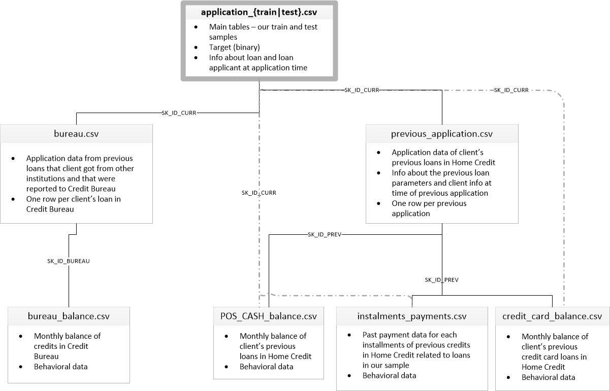
1. 메인 테이블 : application_{train|test}.csv 
   • 고객의 정보와 현재 대출에 대한 정보를 제공한다. 
   • 1이면 미납자, 0이면 성실한 사람
   • SK_ID_CURR
2. 과거 대출 이력 : previous_application.csv
   • 고객의 현재 대출 이전의 과거 대출 정보를 제공한다.
   • SK_ID_PREV, SK_ID_CURR
3. 타사 대출 이력 : bureau.csv
   • 고객의 현재 대출 이전의 타사 대출 정보를 제공한다.
   • SK_ID_BUREAU, SK_ID_CURR
4. 타사 대출 월별 잔액 : bureau_balance.csv
   • Monthly balances of previous credits in Credit Bureau.
   • This table has one row for each month of history of every previous credit reported to Credit Bureau – i.e the table has (#loans in sample * # of relative previous credits * # of months where we have some history observable for the previous credits) rows.
5. 과거 대출의 월별 현금 대출 잔액 : POS_CASH_balance.csv
   • Monthly balance snapshots of previous POS (point of sales) and cash loans that the applicant had with Home Credit.
   • This table has one row for each month of history of every previous credit in Home Credit (consumer credit and cash loans) related to loans in our sample – i.e. the table has (#loans in sample * # of relative previous credits * # of months in which we have some history observable for the previous credits) rows.
6. 과거 대출의 월별 카드 대출 잔액 : credit_card_balance.csv
   • Monthly balance snapshots of previous credit cards that the applicant has with Home Credit.
   • This table has one row for each month of history of every previous credit in Home Credit (consumer credit and cash loans) related to loans in our sample – i.e. the table has (#loans in sample * # of relative previous credit cards * # of months where we have some history observable for the previous credit card) rows.
7. 과거 대출의 월별 납부 이력 : installments_payments.csv
   • Repayment history for the previously disbursed credits in Home Credit related to the loans in our sample.
   • There is a) one row for every payment that was made plus b) one row each for missed payment.
   • One row is equivalent to one payment of one installment OR one installment corresponding to one payment of one previous Home Credit credit related to loans in our sample.
8. HomeCredit_columns_description.csv

 

 

 

주요 분석 도메인 : 고객 자산, 고객 소득, 고객 거주지, 고객의 행동, 타기관 대출 이력, 과거 대출 납부 이력, 과거 대출 이력, 고객 신상(성별, 직장 유무), 대출 금액, 신용 점수 등

 

application_train(test) 시각화 및 Preprocessing

Data load

import numpy as np
import pandas as pd
import gc
import time
import matplotlib.pyplot as plt
import seaborn as sns
#import warning
%matplotlib inline

#warning.ignorewarning(...)

pd.set_option('display.max_rows', 100)
pd.set_option('display.max_columns', 200)

 

app_train = pd.read_csv('/home/soon5770/Kaggle/home-credit-default-risk/application_train.csv')
app_test = pd.read_csv('/home/soon5770/Kaggle/home-credit-default-risk/application_test.csv')

 

app_train.head()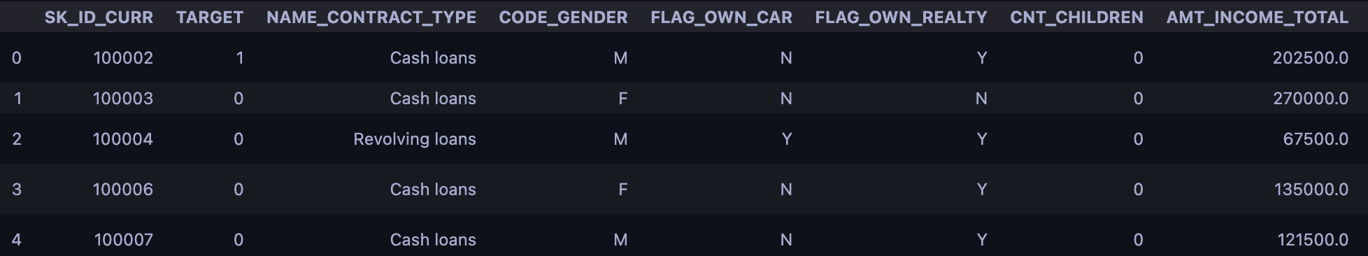

 

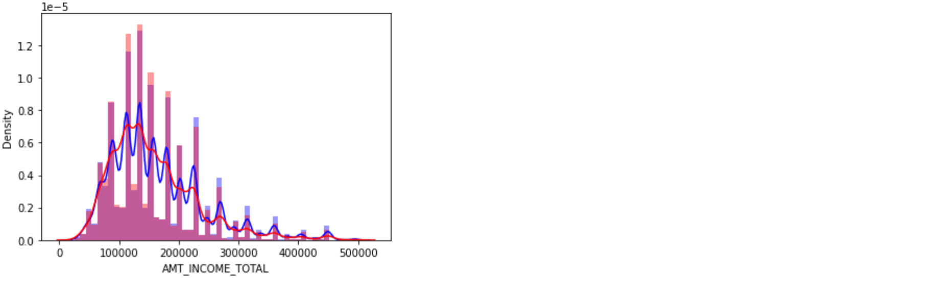
TARGET 값에 따른 AMT_INCOME_TOTAL값 분포도 비교

• distplot과 violinplot 시각화
• plt.subplots() 기반으로 seaborn의 distplot과 violinplot으로 분포도 비교 시각화

cond1 = (app_train['TARGET']==1)
cond0 = (app_train['TARGET']==0)
cond_amt = (app_train['AMT_INCOME_TOTAL']<500000)

sns.distplot(app_train[cond0 & cond_amt]['AMT_INCOME_TOTAL'], label='0', color='blue')
sns.distplot(app_train[cond1 & cond_amt]['AMT_INCOME_TOTAL'], label='1', color='red')

 

 

sns.violinplot(x='TARGET', y='AMT_INCOME_TOTAL', data=app_train[cond_amt])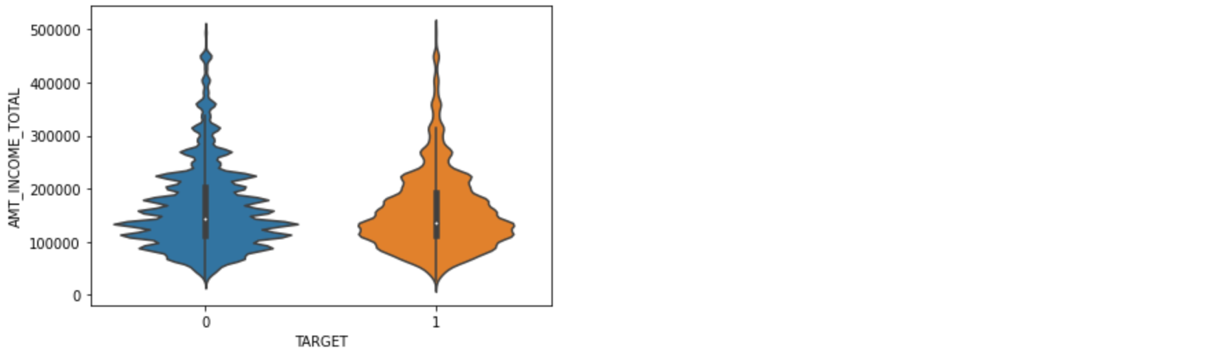

 

한 번에 그리기

fig는 전체 그림을 말하고, axs는 각각의 subplot의 축을 말한다.

위의 코드에 ax 지정만 해주면 된다.

cond1 = (app_train['TARGET']==1)
cond0 = (app_train['TARGET']==0)
cond_amt = (app_train['AMT_INCOME_TOTAL']<500000)

fig, axs = plt.subplots(figsize=(12,4), nrows=1, ncols=2, squeeze=False) # 1행 2열의 subplot 만들기

sns.violinplot(x='TARGET', y='AMT_INCOME_TOTAL', data=app_train[cond_amt], ax=axs[0][0])
sns.distplot(app_train[cond0 & cond_amt]['AMT_INCOME_TOTAL'], label='0', color='blue', ax=axs[0][1])
sns.distplot(app_train[cond1 & cond_amt]['AMT_INCOME_TOTAL'], label='1', color='red', ax=axs[0][1])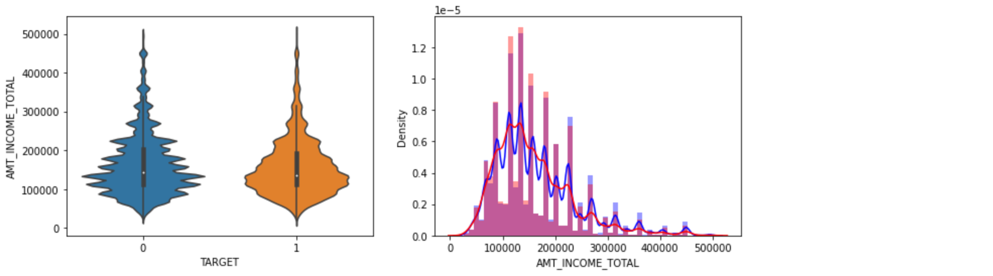

 

위 코드를 함수화 해보자

def show_column_hist_by_target(df, column, is_amt=False):
    cond1 = (df['TARGET'] == 1)
    cond0 = (df['TARGET'] == 0)
    
    fig, axs = plt.subplots(figsize=(12,4), nrows=1, ncols=2, squeeze=False) # 1행 2열의 subplot 만들기

    cond_amt = True
    if is_amt:
        cond_amt = df[column] < 500000
    
    sns.violinplot(x='TARGET', y=column, data=app_train[cond_amt], ax=axs[0][0])
    sns.distplot(app_train[cond0 & cond_amt][column], label='0', color='blue', ax=axs[0][1])
    sns.distplot(app_train[cond1 & cond_amt][column], label='1', color='red', ax=axs[0][1])

show_column_hist_by_target(app_train, 'AMT_INCOME_TOTAL', is_amt=True)

 

app_train과 app_test를 합쳐서 한번에 데이터 preprocessing 수행

train data에 데이터를 추가할건데 또 같은 로직으로 test data를 만들기 귀찮기 때문에 train data와 test data를 합친다.

그리고 다시 분리한다.

target이 있는 데이터가 train data이고, target이 없는 데이터가 test data 이다.

app_train.shape, app_test.shape

((307511, 122), (48744, 121))

 

apps = pd.concat([app_train, app_test])
apps.shape

(356255, 122)

 

Object feature 들을 Label Encoding

Light GBM 같은 추리계열에서는 Label Encoding이 더 좋다.

pandas의 factorize() 이용 : 한번에 한 컬럼만 적용이 가능하므로 루프를 돌려야 한다.

 

apps.dtypes[apps.dtypes == 'object']

 

object_columns = apps.dtypes[apps.dtypes == 'object'].index.tolist()

for column in object_columns:
    apps[column] = pd.factorize(apps[column])[0] # 앞에것을 가져오므로 [0]

 

Null 값 일괄 변환

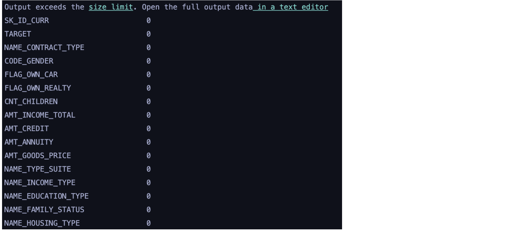
null 값 확인하기

apps.isnull().sum().head(100)

 

 

-999로 모든 컬럼들의 Null값 변환

apps = apps.fillna(-999)

 

다시 null 값을 확인하면 

null 값이 없는 걸 확인할 수 있다.

 

train, test 데이터 다시 분리

app_train = apps[apps['TARGET'] != -999]
app_test = apps[apps['TARGET'] == -999]
app_train.shape, app_test.shape

((307511, 122), (48744, 122))

 

 

잘 분리 되었지만 여기서 test 데이터는 target 값이 떨어져 나가야 한다.

app_test = app_test.drop('TARGET', axis=1, inplace=False)
app_test.shape

(48744, 121)

 

.