목차
- 가중치 초기화 (Weight Initialization)
- 좋은 가중치 초기화 조건
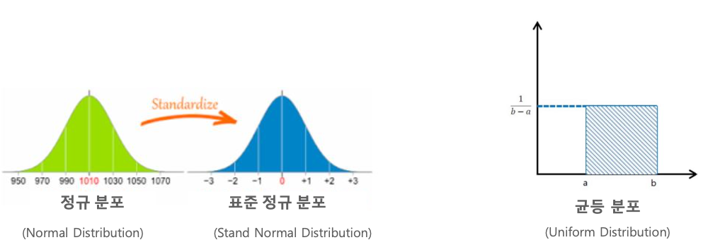
- 평균이 1 이고 표준편차가 1인 표준 정규분포에서 난수 추출
- 표준 편차 변경에 따른 Sigmoid 출력 결과
- Xavier Glorot Initialization
- Xavier initialization - 정규분포(glorot_normal), 균일분포(glorot_uniform)
- He Initialization
- Weight Initialization을 He Normal로 변경 후 성능 검증
가중치 초기화 (Weight Initialization)
좋은 가중치 초기화 조건
- 값이 동일해서는 안된다.
- 충분히 작아야 한다.
- 적당한 분산(또는 표준편차)를 가져야 한다.
충분히 작을 수 있도록 도와주기 위한 적당한 분산.
평균이 1 이고 표준편차가 1인 표준 정규분포에서 난수 추출
- 표준 편차가 클수록 개별 값의 크기가 일반적으로 커진다.
# 표준 정규분포에서 난수 추출
numbers = np.random.normal(loc=0.0,scale=1,size=[100, 100])
# location(위치)=평균, scale=표준편차, size=2차원행렬
print(numbers)
print(numbers.mean())
print(numbers.std())
print(numbers.sum())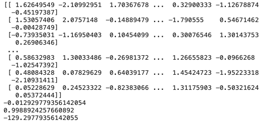
평균은 거의 0이고, 표준편차는 거의 1인 것을 확인할 수 있다.
표준 편차 변경에 따른 Sigmoid 출력 결과
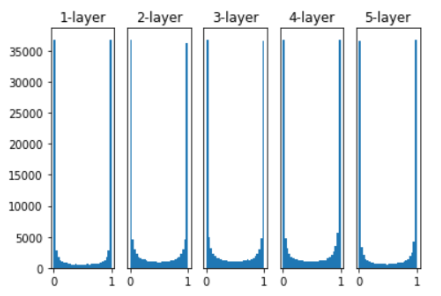
평균 0, 표준편차 1 인 표준 정규 분포에서 Weight 초기화 시,
Sigmoid 출력이 대부분 0과 1로 수렴한다.
입력값이 -∞ 로 가던가 +∞ 로 가던가
음수로 크거나 양수로 크거나 하는 바람에, 값이 다 0, 1 이렇게 나온다.
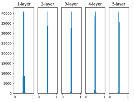
평균 0, 표준편차 0.01 인 표준 정규 분포에서 Weight 초기화 시, Sigmoid 출력은 대부분 0.5로 수렴한다.
표준편차를 작게하면 0.5로 몰리게 된다.
Xavier Glorot Initialization
입력 노드와 출력 노드의 개수를 감안하여 동적으로 Weight를 초기화 하는 것이 좋다.
fan in과 fan out으로 표준편차를 동적으로 개선해보자!
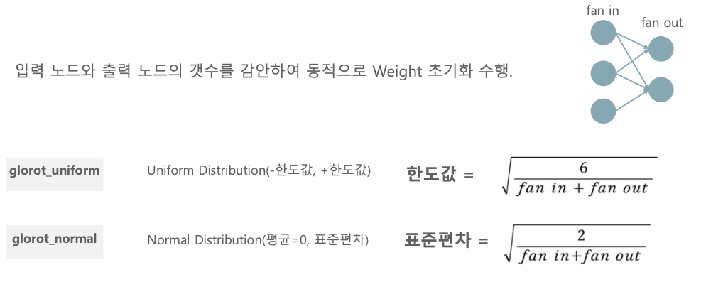
fan in : weight에 곱해지는 입력의 노드의 개수
fan out : 출력 노드의 개수
직관적으로 봤을 때, fan in과 fan out의 개수가 많다면 표준편차는 작아지게 된다.
이렇게 fan in과 fan out으로 크기에 따라 표준편차를 동적으로 조절하는 방법이다.
Xavier initialization - 정규분포(glorot_normal), 균일분포(glorot_uniform)
# glorot_normal
fan_in = 10
fan_out = 8
scale_value = np.sqrt(2/(fan_in + fan_out))
print('scale:', scale_value)
weights = np.random.normal(loc=0.0, scale=scale_value, size=(100, 100))
print(weights)
print('weights mean:',weights.mean(), 'std:', weights.std(), 'sum:', weights.sum())
위에서 진행한 일반적인 난수와 비교했을 때, 보다 값 자체의 크기가 작은 것을 확인할 수 있다.
변동성이 좀더 작다.
scale_value (표준편차)가 작기 때문이다.
# glorot_uniform
fan_in = 10
fan_out = 8
limit = np.sqrt(6/(fan_in + fan_out))
print('limit:', limit)
weights = np.random.uniform(-1*limit, limit, size=(100, 100))
print(weights)
print('weights mean:',weights.mean(), 'std:', weights.std(), 'sum:', weights.sum())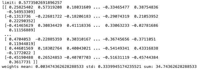
균일 분포에서 랜덤값을 뽑아내면 normal distribution에서 보다 약간 크다.
결국은 표준편차가 매우 작은 0.01 에서 큰 1 사이에서, fan in과 fan out을 통해 균형을 잡는 것이다.
이 입력 노드와 출력 노드 개수가 많으면 표준편차가 작아지게 된다.
He Initialization
자비에르 방식은 주로 시그모이드나 하이퍼볼릭 탄젠트에 최적화 되어 있다면, He는 ReLU에 최적화 된 가중치 최적화 방법이다.
자비에르 방식과 크게 다르지 않다.
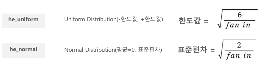
fan in 만 이용하기 때문에 분포(표준편차)가 자비에르 방식보다 조금 크다.
# he_nromal
fan_in = 10
fan_out = 8
scale_value = np.sqrt(2/(fan_in))
print('scale:', scale_value)
weights = np.random.normal(loc=0.0, scale=scale_value, size=(100, 100))
print(weights)
print('weights mean:',weights.mean(), 'std:', weights.std(), 'sum:', weights.sum())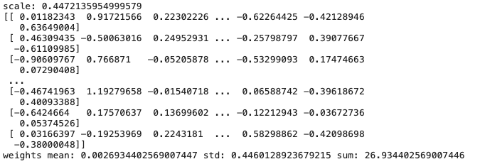
Weight Initialization을 He Normal로 변경 후 성능 검증
- Keras Conv2D의 기본 weight 초기화는 glorot_uniform임. 이를 he_normal로 변경 후 동일 모델로 성능 테스트
- label은 원-핫 인코딩을 적용
from tensorflow.keras.datasets import cifar10
from tensorflow.keras.utils import to_categorical

def get_preprocessed_data(images, labels):
    # 학습과 테스트 이미지 array를 0~1 사이값으로 scale 및 float32 형 변형.
    images = np.array(images/255.0, dtype=np.float32)
    labels = np.array(labels, dtype=np.float32)
    labels = labels.squeeze()

    return images, labels

# 0 ~ 1사이값 float32로 변경하는 함수 호출 한 뒤 OHE 적용
def get_preprocessed_ohe(images, labels):
    images, labels = get_preprocessed_data(images, labels)
    # OHE 적용
    oh_labels = to_categorical(labels)
    return images, oh_labels

(train_images, train_labels), (test_images, test_labels) = cifar10.load_data()

train_images, train_oh_labels = get_preprocessed_ohe(train_images, train_labels)
test_images, test_oh_labels = get_preprocessed_ohe(test_images, test_labels)
print(train_images.shape, train_oh_labels.shape, test_images.shape, test_oh_labels.shape)
데이터 로드, 전처리, 원핫 인코딩
그 후 kernel_initializer 만 he_normal로 바꾸어준다.
from tensorflow.keras.models import Sequential, Model
from tensorflow.keras.layers import Input, Dense , Conv2D , Dropout , Flatten , Activation, MaxPooling2D , GlobalAveragePooling2D
from tensorflow.keras.optimizers import Adam , RMSprop
from tensorflow.keras.layers import BatchNormalization
from tensorflow.keras.callbacks import ReduceLROnPlateau , EarlyStopping , ModelCheckpoint , LearningRateScheduler

input_tensor = Input(shape=(IMAGE_SIZE, IMAGE_SIZE, 3))

#x = Conv2D(filters=32, kernel_size=(5, 5), padding='valid', activation='relu')(input_tensor)
x = Conv2D(filters=32, kernel_size=(3, 3), padding='same', activation='relu', kernel_initializer='he_normal')(input_tensor)
x = Conv2D(filters=32, kernel_size=(3, 3), padding='same', activation='relu', kernel_initializer='he_normal')(x)
x = MaxPooling2D(pool_size=(2, 2))(x)

x = Conv2D(filters=64, kernel_size=3, padding='same', activation='relu', kernel_initializer='he_normal')(x)
x = Conv2D(filters=64, kernel_size=3, padding='same', kernel_initializer='he_normal')(x)
x = Activation('relu')(x)
x = MaxPooling2D(pool_size=2)(x)

x = Conv2D(filters=128, kernel_size=3, padding='same', activation='relu', kernel_initializer='he_normal')(x)
x = Conv2D(filters=128, kernel_size=3, padding='same', activation='relu', kernel_initializer='he_normal')(x)
x = MaxPooling2D(pool_size=2)(x)

# cifar10의 클래스가 10개 이므로 마지막 classification의 Dense layer units갯수는 10
x = Flatten(name='flatten')(x)
x = Dropout(rate=0.5)(x)
x = Dense(300, activation='relu', name='fc1')(x)
x = Dropout(rate=0.3)(x)
output = Dense(10, activation='softmax', name='output')(x)

model = Model(inputs=input_tensor, outputs=output)

model.summary()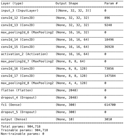
# optimizer는 Adam으로 설정하고, label값이 원-핫 인코딩이므로 loss는 categorical_crossentropy 임.
model.compile(optimizer=Adam(), loss='categorical_crossentropy', metrics=['accuracy'])
history = model.fit(x=train_images, y=train_oh_labels, batch_size=64, epochs=30, validation_split=0.15 )
학습을 하고 결과를 보면
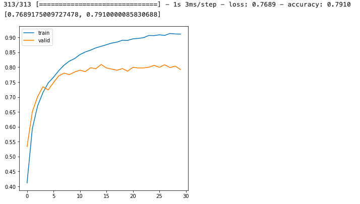
앞에서 한 결과와 큰 차이는 없다.
데이터 by 데이터로 차이가 있을 수는 있겠지만 별 차이는 없다.
'🖼 Computer Vision > CNN' 카테고리의 다른 글
| CNN - Global Average Pooling (0) | 2022.03.04 |
|---|---|
| CNN - Batch Normalization (0) | 2022.03.03 |
| CIFAR10 (0) | 2022.03.03 |
| CNN - Convolution 연산 후 Feature map 크기 계산 이해하기 (0) | 2022.03.02 |
| CNN - Convolution 연산에서 Filter에 대한 이해 (3) | 2022.03.02 |